
The Internet has become an indispensable part of our lives, and it is of vital importance to work out how to guarantee the security of users’ sensitive information and privacy in cyberspace. Most of the Internet traffic is encrypted with Transport Layer Security (TLS), which cannot guarantee absolute security. Malware has been seen to use TLS to communicate with their command server, either to receive instructions from the server or to send back sensitive data collected from the infected host. Given how ubiquitous TLS has become and how cheap and easy it is nowadays to obtain valid TLS certificates, the amount of malware that uses TLS will keep increasing. Therefore, it is necessary to detect encrypted TLS communication traffic in malware.
Characteristics of Malware
Many deficiencies have been found in the method of detecting malware communication by decrypting TLS packet payloads. This paper focuses on packets’ metadata rather than on packets’ contents to avoid shortcomings of malware detection based on payload decryption.
The selection of features must be motivated by clear differences in the characteristics of observed malicious and benign flows. If both datasets are very similar in the first place, trying to classify flows would most certainly fail. Studying distinct characteristics between data can verify that malicious and benign flows are separable and has certain guiding significance for feature construction and selection.
The report[1] written by Olivier Roques of Imperial College London conducted an analysis of the feature distribution of a dataset[2]. The dataset contained over 10,000 malware flows and over 20,000 benign flows. These benign flows were collected from Lastline’s office network environment from May to June 2019. Malware flows were spread from 2016 to 2019 and mainly came from MTA[3] and Stratosphere[4], two datasets publicly available. This paper enumerates some differences between malware and benign TLS flows from the aspects of metadata, TLS parameters, and certificates.
1. Metadata
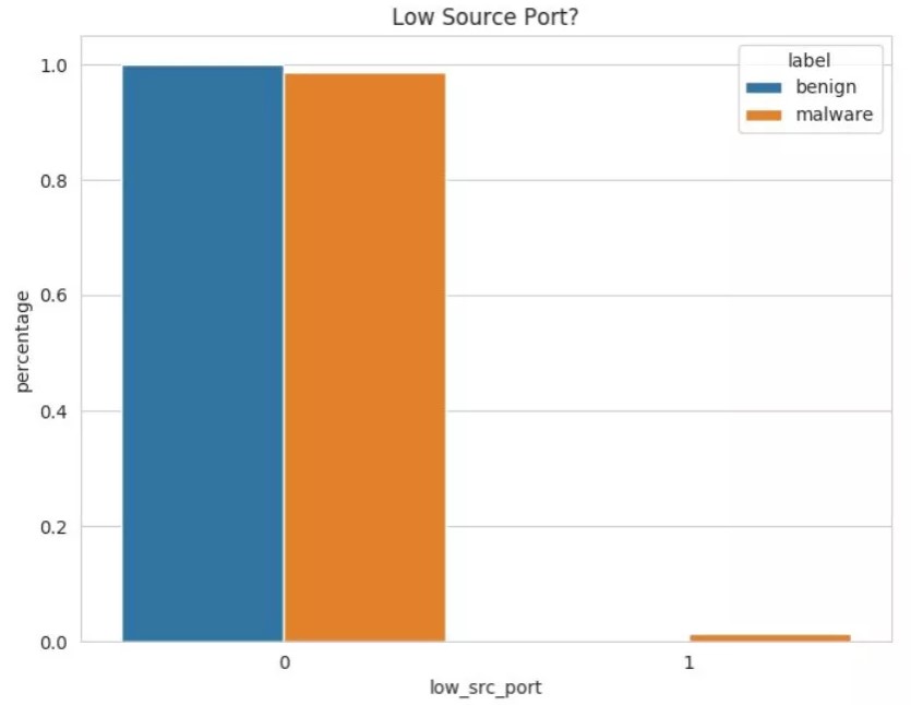
Source port: By default, operating systems (OSs)assign source ports randomly in the range 49152–65535. However, some malware families do not request a source port from the OS, but uses a custom one, which makes them stand out among normal connections. As shown in the following figure, the horizontal axis indicates whether a source port is randomly assigned by the system, and the vertical axis indicates the percentages of malware and benign flows.
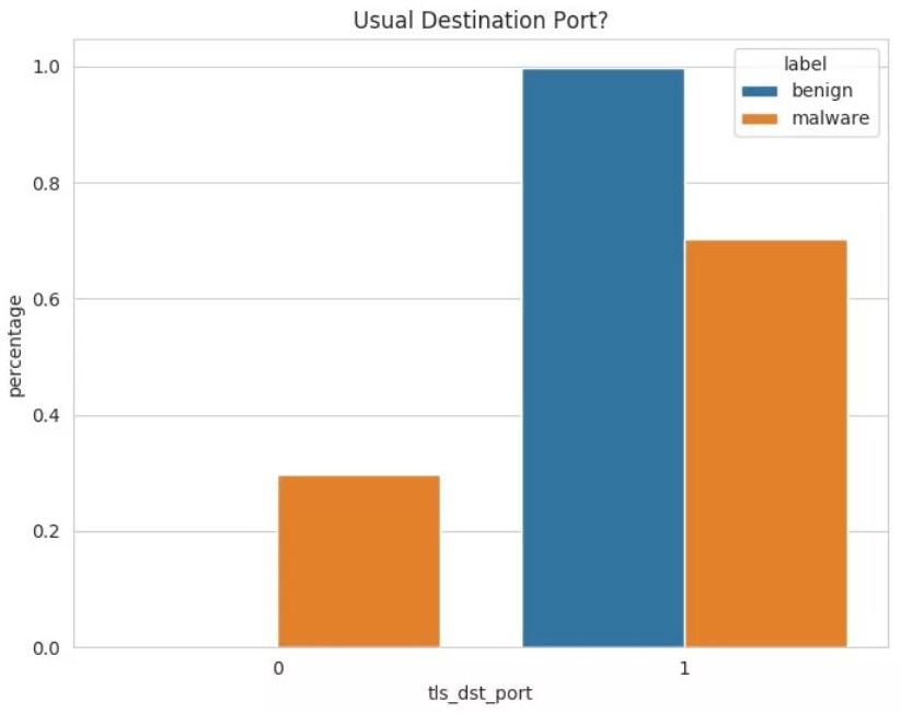
Destination port: By default, legitimate servers listen on specific ports (such as port 443, 465, 853, and 992) for TLS-related packets, and apart from malware there is no reason for clients to initiate TLS sessions to other ports. Nevertheless, some malware authors may just want to use encryption and do not care about which ports their server should use. Thus, these malware samples use other ports to provide TLS services, which makes them more prone to being blocked or detected. As shown in the following figure, the horizontal axis indicates whether a destination port is a usual TLS port, and the vertical axis indicates the percentages of malware and benign flows.
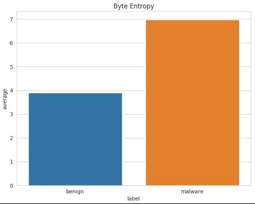
Byte entropy: High entropy results from the use of strong encryption and where we could have expected malware flows to have less entropy due to maybe ignoring encryption of data packets, it is the contrary that happens. As shown in the following figure, the horizontal axis indicates malware and benign flows, and the vertical axis indicates the average byte entropy. We speculate that this is correlated to the short flow duration of benign sessions: Since the TLS handshake is not encrypted and accounts for a larger portion of the benign TLS session, it lowers the final average entropy.
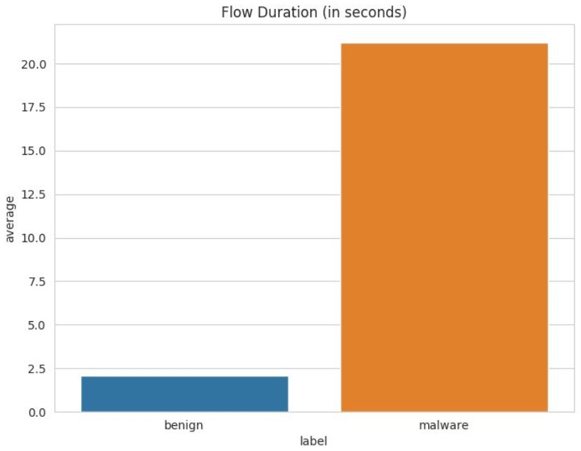
Flow duration: As shown in the following figure, the horizontal axis indicates malware and benign flows, and the vertical axis indicates the flow duration. Malicious communications collected last longer in average than benign ones. This is due to the fact that Lastline’s employees typically use TLS to load web pages and download small resources which results in short-lived TLS sessions, whereas malware may tend to send and receive a larger amount of data.
2. TLS Parameters
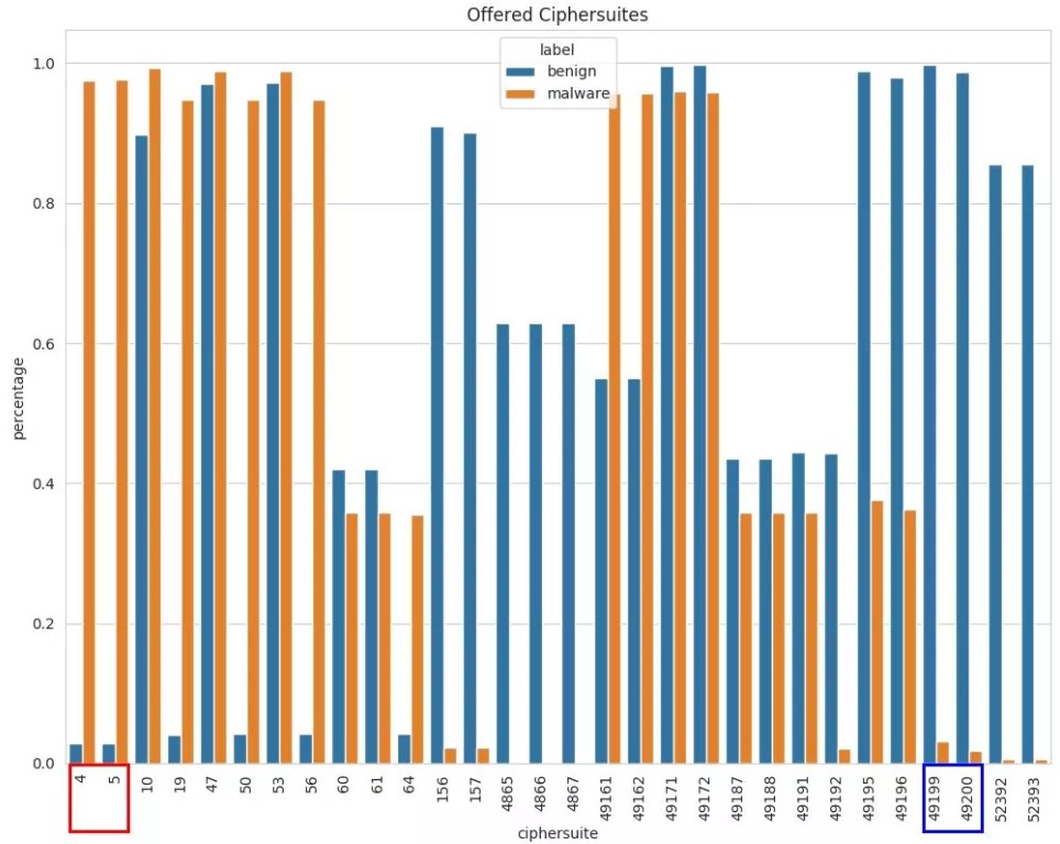
Ciphersuites offered by TLS clients: As shown in the following figure, the horizontal axis indicates the code of a TLS ciphersuite, and the vertical axis indicates the percentages of malware and benign flows in each ciphersuite. Some ciphersuites are completely ignored by malware, while others are disproportionally favored. For example, the two ciphersuites in the blue box are mostly used by benign flows by virtue of security, and another two in the red box are mainly used by malware but considered by benign flows to be insecure for adopting the outdated RC4 algorithm. This may be because malware authors lack the awareness of choosing strong ciphersuites or updating ciphersuites or are only concerned about content encryption rather than algorithm choices.
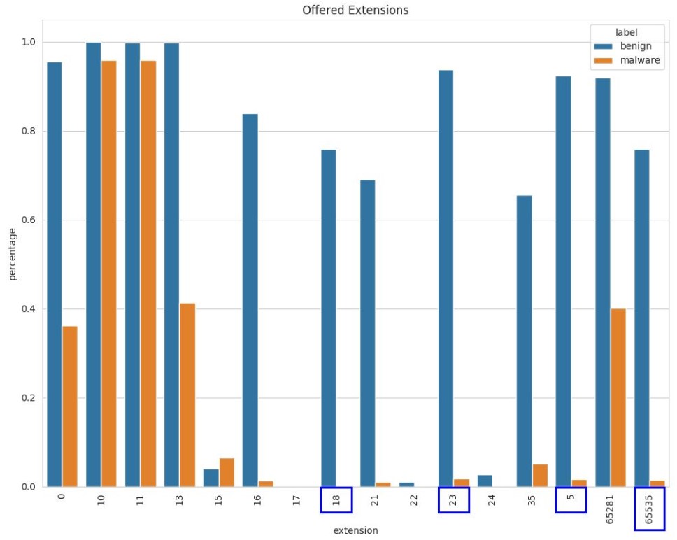
Extensions offered by TLS clients: As shown in the following figure, the horizontal axis indicates the code of a TLS extension, and the vertical axis indicates the percentages of malware and benign flows in each extension. Compared with malware, benign flows tend to offer more extensions. Extensions in the following blue boxes are barely used by malware.
3. Certificate Differences
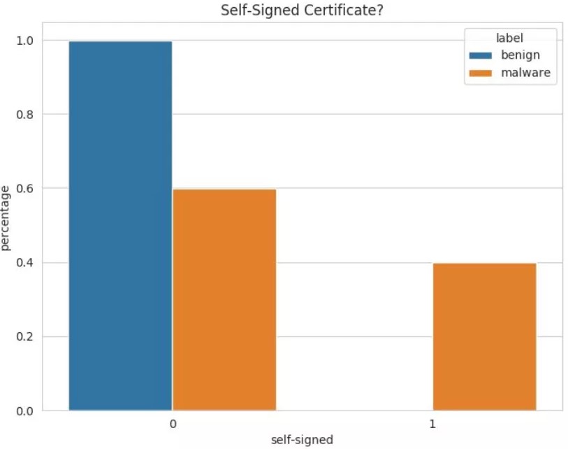
Whether a certificate is self-signed: As shown in the following figure, the horizontal axis indicates whether a certificate is self-signed, and the vertical axis indicates the percentages of malware and benign flows in a self-signed certificate. As expected, malware tend to rely a lot more on self-signed certificates.
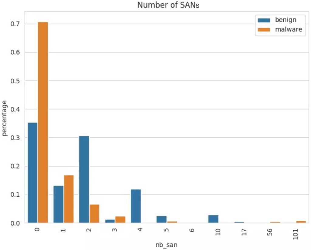
Number of Subject Alternative Names (SANs) contained by a certificate: As shown in the following figure, the horizontal axis indicates the number of SANs, and the vertical axis indicates the percentages of malware and benign flows of certificates containing different numbers of SANs. In contrast with malware, benign flow certificates contain a small number of SANs. A possible explanation would be that legitimate certificates from reputable sources are expensive, so there are incentives for companies to put multiple domains in a single certificate.
Through the exploration and research into malware communication traffic detection, we can discuss related issues from the following aspects.
4. Data Collection
The performance of a classifier greatly depends on the quality of training datasets. It can also be seen from the preceding section that many features lie on the method or environment of dataset acquisition. Henceforth, we need to create a dataset that reflects current network traffic as much as possible. As for datasets, the author thinks that the use of a classifier in actual scenarios is mainly influenced by the following two factors:
(1) Network environment
In general, malicious traffic is similar in different network environments, while benign traffic is greatly affected by network environments and will have major changes with different operating systems, browsers, and business scenarios. For example, schools, homes, and different enterprises generate different traffic.
To reduce the number of false positives, we need to create different benign datasets for different environments. Fortunately, it is easy to collect benign data.
(2) Time
Compared with benign traffic, malicious traffic is more affected by temporal bias. The data collected is subject to concept drifting, meaning that data becomes obsolete over time. Malware is constantly optimized and updated, new malware is introduced, users’ habits change, etc. The availability of trained models is limited in time, and these models are likely to be effective only in the near future.
There is still something that we can do to overcome the deviation of data over time. On the one hand, in order to avoid the influence of temporal bias, we should collect both malicious and benign data generated during the same period to ensure that the classifier learns the features of black and white data rather than the differences between traffic generated at different times. On the other hand, to make the classifier robust against time decay, we need to stay tuned to new malware, keep malicious datasets updated, or combine concept drifting sample detection to enable the classifier to detect new threats.
5. Feature Construction and Selection
Feature engineering is a process of transforming raw data into model training data. Good feature engineering can improve model performance and sometimes can even achieve good results on simple models. Feature engineering generally includes three parts: feature construction, feature extraction, and feature selection. The author briefly describes the related issues of feature construction and feature selection in malware traffic detection.
(1) Feature construction
TLS parameters, such as ciphersuites and extensions, can be set. Some attackers will also continuously update malware based on parameters widely used in legitimate traffic. Certificate parameters, such as whether the certificate is self-signed and when the certificate expires, can also be modified in certain ways. Therefore, these features are easily affected by datasets or time.
Compared with these changeable features, meta-features, such as the number of bytes, the number of packets, and byte distribution of data flows, are not directly controlled by attackers and are difficult to be tampered with. Therefore, they are more distinguishable and robust. We can try to find and use such features. More importantly, in order to prevent attackers from modifying parameters to make the classifier unable to distinguish the parameters, it is necessary to keep the features used by the classifier secret.
(2) Feature selection
Generally speaking, the more valid features there are, the better detection effects are. To improve robustness, the classifier can take into account features from other types of flows rather than limit itself to TLS. For instance, it can extract more features by combining DNS queries made prior to the TLS handshake or HTTP flows originating from the same source IP address.
However, as features increase, the classifier consumes more and more time and space. It is necessary to strike a balance between accuracy and resource consumption according to the actual situation and to simplify or expand the feature set in a timely manner.
6. Model Selection
Data and features determine the upper limit of machine learning models’ performance, and models and algorithms just approach this upper limit. It is a common practice to compare different models on the same dataset and select the best model based on detection results on test sets. Whether the results are good or bad, in fact, the difference between the results of most models that fit application scenarios is not very large. The author thinks it important to select the appropriate model and select and optimize model parameters, which, however, is not decisive to detection results.
7. Balance Between the Recall Rate and False Positive Rate
It is important to have a high recall rate, but the number of false positives is a key factor in determining whether the detection system is available. In high traffic scenarios, even if the false positive rate is quite low, the number of false positives can be very large. Regardless of the recall rate, these false positives will take up the energy and time of operations personnel, which will become a management burden and might even cause legitimate positives to be ignored. Thus, it is necessary to strike a good balance between the recall rate and the false positive rate or take control of both rates according to actual needs.
8. False Positives in the Current Network Environment
When models are used in the current network environment, causes of false positives are complicated. Overfitting or underfitting on training sets may cause false positives. We need to focus on data collection and feature engineering or use some other methods to mitigate false positives. Firstly, tune policies, for example, by increasing the threshold to ensure higher accuracy and thereby reduce false positives. Secondly, use expert knowledge and experience, such as regularly conducting secondary analysis or post-processing of model output results and correcting model output results to reduce false positives. Lastly, since using the classifier alone will inevitably produce false positives, we can combine the classifier with other detectors or methods, such as the DGA detector or JA3 method, to reduce false positives, or use active detection technology at the same time to discover threats in the network environment.
9. Sum-up
This paper lists some differences between malware and benign TLS flows and discusses critical issues in malware communication traffic detection. Practices show that models constructed by using distinctive features can effectively detect malicious flows from encrypted TLS traffic. Of course, as attackers improve techniques, malware becomes more and more covert. Only by constantly exploring and researching new features and methods can we better cope with increasingly complex attacks in network traffic.
References
[1] https://github.com/ojroques/tls-malware-detection
[2]https://drive.google.com/drive/folders/1TfRz6q65wPaiuB4D9qmyfCxoJ8zEBUQ
[3] BradDuncan. malware-traffic-analysis. URL: https://www.malware-trafficanalysis.net/
[4] Stratosphere IPS. Malware Capture Facility Project. URL: https://www.stratosphereips.org/datasets-malware
